An Overview of Flatgeobuf

As of lately I have been extremely interested in the FlatgeoBuf file format. Flatgeobuf is a file format that falls under the category of cloud native geospatial formats. Such formats organize features in a spatially localized way that allows them to be queried directly from S3 or another similar object store. This helps to reduce both the infrastructure costs and maintenance needed for serving geospatial data on the web.

Flatgeobuf extends the Google FlatBuffers library. Google FlatBuffers is a cross-platform, schema-driven serialization library that enables zero-copy, memory-efficient access to structured binary data without deserialization. In a geospatial application, this format can be utilized to help to reduce the serialization cost of working with large polygons.

FlatGeobuf File Internals

A FlatGeoBuf file consists of a header followed by a sequence of features. The header contains metadata such as the dataset name, feature schema, and coordinate reference system (CRS). It also includes information describing the spatial index, though the index itself is stored separately in the file.

FlatGeoBuf uses a packed Hilbert R-tree as its spatial index. To build this index, the writer computes the bounding box of each feature, then sorts these bounding boxes using a Hilbert space-filling curve before packing them into an R-tree structure. This process ensures that features that are spatially close are also close together in the file’s memory layout, enabling efficient spatial queries and minimizing I/O.

Clients can read the spatial index once and use it to perform efficient range queries against the same FlatGeoBuf file, often via HTTP range requests. For more details on the internals of the file format I recommend this blog post.

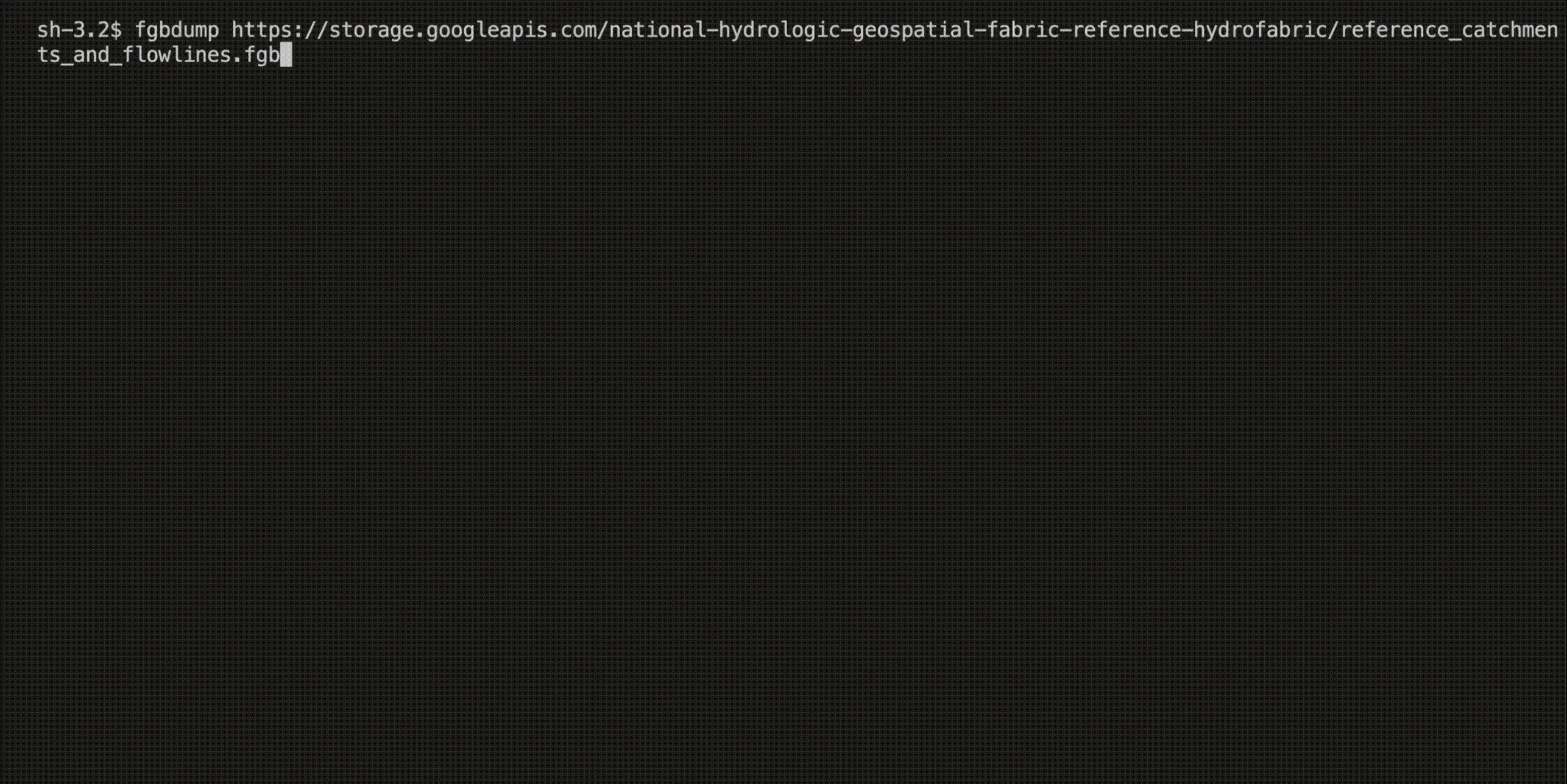
To explore a FlatGeobuf file’s metadata, I recommend utilizing my fgbdump TUI CLI application.

Querying FlatGeobuf

Due to the spatial index, a FlatGeobuf can be queried directly on S3 without needing to download the entire file. It is important to note that FlatGeobuf does not have any B-tree index on properties so you can only do efficient filtering on

1. A bounding box
2. A feature ID (not all clients support this, but it is possible by using parts of the ids in the spatial index; for more info read this)

As a few notes:

• Since the spatial index is calculated by using the bounding box of each feature, some clients may return features outside of the query area due to the fact their associated bounding boxes were inside.
• Although it is generally not recommended to compress your FlatGeobuf file, you can nonetheless use seek optimized zip in GDAL to compress the file in a way that preserves proper spatial locality. For more info read this.
• In order to utilize predicate pushdown with the spatial index, you should ensure that your query client is opening the FlatGeobuf file properly. This is sometimes a bit different depending on the client. Here are a few examples:

duckdb

SELECT *
FROM ST_Read(
    'gcs://national-hydrologic-geospatial-fabric-reference-hydrofabric/reference_catchments.fgb',
    spatial_filter_box = ST_MakeBox2D(
        ST_Point(-108.50231860661755, 39.05108882481538),
        ST_Point(-108.50231860661755, 39.05108882481538)
    )
)

Geopandas

import  geopandas as gpd
url = 'https://storage.googleapis.com/national-hydrologic-geospatial-fabric-reference-hydrofabric/reference_catchments.fgb'
gdf = gpd.read_file(url, engine="fiona", bbox=[-108.50231860661755, 39.05108882481538, -108.50231860661755, 39.05108882481538])

Apache Sedona DB

import sedona.db 

sd = sedona.db.connect()

# Load hydrofabric (catchments + flowlines)
hydro_url = "https://storage.googleapis.com/national-hydrologic-geospatial-fabric-reference-hydrofabric/reference_catchments_and_flowlines.fgb"
sd.read_pyogrio(hydro_url).to_view("hydrofabric")

df = sd.sql("""
SELECT *
FROM hydrofabric
WHERE ST_Intersects(
    wkb_geometry,
    ST_SetSRID(
        ST_Point(-108.50231860661755, 39.05108882481538),
        4326
    )
);
""")

df.show()

Written January 17, 2026